Remember, the goal is not so much to teach you to create a budget, but to help you acquire some spreadsheet skills. Try to follow the directions.

Entering the months

• Click on cell A4
• Type the word, January and press the Enter Key

A heavy line should appear around cell A4 because that is the active cell. There should also be a small square in the lower left corner of the active cell.
The small square is called a Fill Handle

• Move the mouse close to the fill handle until it becomes a plus sign

• Click the left mouse button and hold it down
• Drag the Fill Handle to cell A15
• Let up on the mouse button
  January to December should have filled from cells A4 to A15
  You now know how to use the fill handles to fill data to multiple cells. You can also fill Right.
  (You could also have highlighted the cells and used the Fill Down option from the Edit Menu)

• Click cell D2 and give your budget a title

Entering Budget Categories & Amounts

• Click in cell B3
• Enter budget categories to cell G3
• Click in cell B4
• Enter amounts for each month and category, cells B4 to G15

Entering formulas to total each category

Filling the formula right

We could use the fill handles to fill right the way we filled the months down. Instead we will use a method that does not depend on the mouse.

• Make sure that B17 is the active cell
  Click in it
• Press the F8 Key
• Use the Right Arrow Key to highlight to cell G17
• Hold down the Alt Key and Press E
  To open the Edit Menu
• Select Fill and press Enter
• Select Fill Right and press Enter
  Notice that the formula adjusted for each column. Examine cell C17 and notice that the formula is =SUM(C4:C15)

Totaling all expenditures for the year

• Click cell B1
• Type "Total Expenditures"
• Click cell A1
• Type =SUM(
• Click cell B17
• Select cells B17 to G17
• Type )
  To close the parenthesis
• Press Enter
  You now have a grand total of expenditures for the year

Entering the formula to find the percentage for each expenditure

• Type the word, Percent, in cell A18

We want to divide the total Auto Expenses by the total of all expenses. This will give us the percentage we spent for auto

• Click in cell B18
• Type = (the equal sign)
• Click in cell B17
• Type / (the division sign)
• Click in cell A1
• Press Enter
  The correct percentage should show in B18
• Fill the formula to cell G18 and you will get ERR messages. Why ?

B18 is OK but if we try to fill right we will have a problem. Remember how the formulas adjust themselves when we fill. Cell B18 says =B17/A1

If we fill right, cell C18 will say =C17/A2. There is no number in A2. We need A1 to remain the fixed divisor in each formula. Here is how we do it …

• Click in cell B18
• Edit the formula by putting a dollar sign in front of the A and in front of the 1
  The formula in B18 should be =B17/$A$1
• Now you can fill right to cell G18
  B17 will become C17, then D17, etc. but $A$1 will remain constant

Formatting the cells with the Format Menu

• Click in cell B4
• Hold down the left mouse button and select all of the cells from A1 to G17
• Click the Format Menu
• Click Cells
• Click Currency and No Decimals
• Click OK
  The cells are now formatted for currency

Using the Format Painter

• Right click cell B18
• Select Format Cells
• Select Percentage with no decimals
• Click OK
• Click the Painter Icon from the Toolbar
  
• Hold down the left mouse button and select all the cells, B18 to G18
• Let up on the mouse button and the format is copied to each cell

Additional Formatting

• Select cells B3 to G3
• Click the Borders Icon then select Grid

• Select cells A17 to G18
• Right Click anywhere in this area
• Select Format Cells
• Use the various formats to add borders, shading or any other type of formats

• Use the formatting procedures you have learned to add formatting to the rest of your spreadsheet

Saving your spreadsheet

• Click the File Menu
• Click Save As
• Select a location from the Save In box
• Give your file a name in the File name box
• Select a format for your file from the Save as type box. (accept the default Excel)
• You can even click the folder with a star to create a folder in the location you have selected.

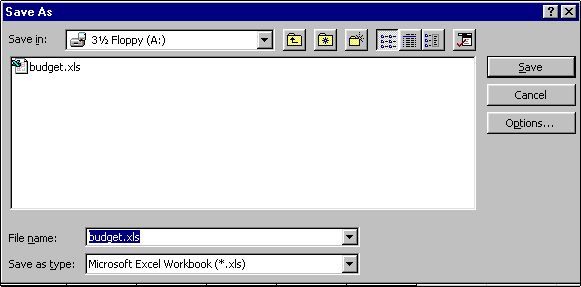
When you are finished, click OK

Inserting a Header

• Click the File Menu and select Page Setup
• Click the Header/Footer tab
• Click Custom Header
• Enter your name on the right side
• Click OK
  You can also select Page Setup from the Print Preview option as below

Printing

• Select Print Preview from the Toolbar